Multimodal Rangefinder for Mapping the Tides of Titan
As a location with the potential to harbor extraterrestrial life within our solar system, accurate information about the conditions on Titan’s (Saturn’s Largest Moon) seas increases our insight of the moon’s geological and atmospheric conditions. In order to navigate the freezing methane seas of the planet, I led a team to develop a RADAR perception system with LiDAR & SONAR recalibration for robust and reliable perception.
Abstract:
In this project, we propose a combined multisensor altimeter system for mapping the tides of Saturn’s Moon, Titan. As a location with the potential to harbor life, accurate information about the conditions on Titan’s liquid hydrocarbon reservoirs increases our insight of the moon’s geological and atmospheric conditions. The mapping system incorporates 3 sensor modalities (RADAR, LiDAR, and SONAR) to ensure robust and high fidelity perception. The RADAR module consists of two 2.4 GHz monopole waveguide antennas, adjusted on a rail to create a Synthetic Aperture RADAR system. An infrared time of flight sensor and an ultrasonic rangefinder serve as a means of enhancing the accuracy and precision of the core RADAR system. In order to evaluate the efficacy of our proposed sensor combination approach, we created an Earth analogue world model designed to emulate key characteristics of Titan’s seas. Our environment utilizes liquid tar with a similar hydrocarbon composition as the liquid methane present on Titan, and incorporates floating dry ice (solid CO2) to emulate potential floating methane icebergs on Titan. We have demonstrated that the rangefinder system functions as intended on man made obstructions, and are in the process of evaluating the system on our Titan analogue. Future work will deal with revisions of the model and rangefinder construction, as well as the potential of digital simulation.


CaSGC? NASA?
The NASA California Space Grant Consortium is a program managed by NASA, the UCSD, and ARC. As project lead, I worked under Dr. Paulo Afonso to create a multi-sensor rangefinder for mapping the tides of titan. I worked alongside Steve Bowman, Joshua Mach, and Edson Munoz. Our work was presented to officials at Kratos Defense & Security Solutions.


RADAR Probe
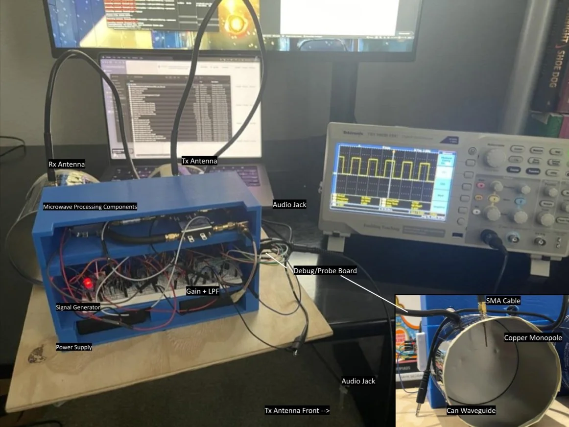
This image showcases the RADAR system I built as Project Lead and sole builder for my NASA CaSGC Research Project. The RADAR probe was designed to construct a visual scene representation of an Earth-analogue of Titan. The transmitting and receiving antennae were made using a 2.5 cm piece of 12 gauge copper to function as a monopole. Although the monopole worked, its range left much to be desired. To enable a larger map, I increased the directivity of the signal by cutting two coffee cans to size for a waveguide, increasing the range from 3m to 35m. The microwave and circuit components were housed in a 3D printed structure for easy access and debug. On the side of the main box, I have a debug board housed, which has connections to the ramp output, signal output, signal received, and ground line. This enabled me to measure each signal using an oscilloscope. The output of the RADAR is the audio jack, which feeds two channel audio into the computer, which I was able to process on Matlab.

Video & Sync Graph
The graph to the right is the raw audio recording that the RADAR system produces. The blue line corresponds to the Sync-Pulse Output from the signal generator, while the red line corresponds to the output from the Low Pass Filter. As the voltages indicate, the Sync Pulse line is the reference signal (which powers the transmitting antenna), while the output from the Low Pass Filter is the appropriately amplified signal measured by the receiving antenna. By comparing these signals, I was able to determine the location of obstructions around the antenna and construct a map based on the SAR methodology. While I had initially hoped to plug the RADAR directly into my laptop and process the audio file, it wasn't so simple: because the laptop didn’t have an audio jack for stereo audio, I had to use an old DSLR Camera we had at home. After recording a “video” on the camera with the RADAR as the audio input, I would transfer the file over to my laptop, and convert it into an audio file for use.

Circuit Diagram
The left diagram shows the three main portions of the RADAR circuitry (inspired by the MIT Lincoln Lab Small RADAR). The signal generator produces 25 KHz Square Waves for the Tx antenna. In order to ensure optimal signal transmission, I incorporated a custom configured RF oscillator and attenuator responsible for impedance matching the signal and facilitating lossless communication. After the Rx antenna records the reflected signal, it passes through a gain stage amplifier and a 15 KHz low pass filter. The switch blots audio transmission, helping the code identify breaks in data. I used variable resistors to tune the electronics, but I did not have a signal generator to calibrate the Rx signal processor. To overcome this challenge, I used Matlab to plot a target waveform, and created an audiofile from the data points, which I was able to connect to the circuit, and use as the reference signal.

SAR Image
This image shows the first SAR Graph that I obtained during testing. Although the antenna receives data up to 350 ft, the signal past 150 ft is effectively noise. Within the range, the antenna successfully identified the wall and the sloped grass hill ahead. The principle behind SAR (synthetic aperture radar) is to compose images captured from a moving antenna, enabling a physically small antenna to be used to map out a large area. To mark the motion of the radar (2” at a time) for the data, I used the blotting switch to break the output signal. Using the RMA SAR Algorithm written by Dr. Gregory L. Charvat from Michigan State University as a reference, I wrote an algorithm in Matlab to process the raw video and sync outputs into a map, increasing fidelity through SONAR & LiDAR sensor-fusion. My algorithm scans for movements of the antenna, using the radiation profile to find the distance of objects at that point. The algorithm generates the map by merging this data.